概述
本文通过代码感受 过拟合
关键代码
注意
训练数据与验证数据格式必须一致
图像都进行归一化
label都进行独热编码(或者都不进行独热编码)
添加多层
model.add(tf.keras.layers.Flatten(input_shape=(28,28)))

model.add(tf.keras.layers.Dense(128,activation='relu'))
model.add(tf.keras.layers.Dense(128,activation='relu'))
model.add(tf.keras.layers.Dense(128,activation='relu'))

model.add(tf.keras.layers.Dense(10,activation='softmax'))
在测试集上验证
每次训练时,在测试集上做验证,通过history可以查看,在测试集上验证的损失情况 和 正确率
model.compile(optimizer=optimizer,loss='categorical_crossentropy',metrics=['acc'])
'''
每次训练时,在测试集上做验证,通过history可以查看,在测试集上验证的损失情况 和 正确率
'''
history=model.fit(train_image,train_label_onehot,epochs=10,
validation_data=(test_image,test_label_onehot))
将训练损失、验证损失画成图像
# 过拟合图像
history.history.get('loss')
plt.plot(history.epoch,history.history.get('loss'),label='loss')
plt.plot(history.epoch,history.history.get('val_loss'),label='val_loss')
plt.legend()
plt.show()
执行结果如下:
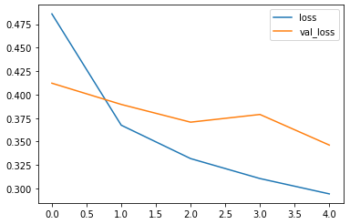
结论:
训练的损失值 一直在 下降
测试集 上验证的 损失值 下降后,又上升了
将训练正确率、验证正确率画成图像
# 过拟合图像
plt.plot(history.epoch,history.history.get('acc'),label='acc')
plt.plot(history.epoch,history.history.get('val_acc'),label='val_acc')
plt.legend()
plt.show()
执行如下:
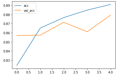
结论:
训练的正确率 一直 上升
测试集 上验证的 正确率有上升,也有下降
代码
加载数据
import tensorflow as tf

(train_image,train_label),(test_image,test_label)=tf.keras.datasets.fashion_mnist.load_data()
其中 训练 数据有 60000 张图像,测试 数据有 10000 张图像
查看图像数据形状
# 查看形状
print(train_image.shape)

print(test_image.shape)
结果:
(60000, 28, 28)
(10000, 28, 28)
训练数据 有60000个,图像是 28宽 28高,也就是说每个图像有28*28=784个特征
也就是说,在神经网络模型中,输入值 共有 784 个
测试数据 有10000个,图像是 28宽 28高
显示图像
通过matplotlib显示图像
# 显示第一张图像

plt.imshow(train_image[0])
分析图像数据
print(train_image[0].shape)
# 查看最大值
np.max(train_image[0])
图像数据,是0-255之间的RGB值
查看类别数据形状
print(train_label.shape)

print(test_label.shape)
执行结果:
(60000,)
(10000,)
分析类别数据
train_label
类别是数字,每个数字对应一个类别,上面有对应表格,共有10个类别
也就是说,在神经网络模型中,输出层 有 10个 感知机(神经元)
对类别进行独热编码
train_label_onehot=tf.keras.utils.to_categorical(train_label)
print(train_label[0])
print(train_label_onehot[0])

test_label_onehot=tf.keras.utils.to_categorical(test_label)
print(test_label[0])
print(test_label_onehot[0])
图像数据 归一化
将图像0-255的RGB转换成0-1的数据
train_image=train_image/255
test_image=test_image/255

train_image[0]
建立模型
model=tf.keras.Sequential()

# 线性回归中是一维数据,而图像数据是二维数据,需要将二维数据转换成一维数据
model.add(tf.keras.layers.Flatten(input_shape=(28,28)))
# 多添加几层,体验过拟合

model.add(tf.keras.layers.Dense(128,activation='relu'))
model.add(tf.keras.layers.Dense(128,activation='relu'))
model.add(tf.keras.layers.Dense(128,activation='relu'))

# 10个分类,softmax的作用就是将10个输出值变成概率值,这些概率值之和为1
model.add(tf.keras.layers.Dense(10,activation='softmax'))

model.summary()
配置训练模型
由于目标值 分类 是 one-hot 独热编码 ,所以使用 categorical_crossentropy 损失函数
optimizer=tf.keras.optimizers.Adam()
model.compile(optimizer=optimizer,loss='categorical_crossentropy',metrics=['acc'])
开始训练
每次训练时,在测试集上做验证,通过history可以查看,在测试集上验证的损失情况 和 正确率
'''
每次训练时,在测试集上做验证,通过history可以查看,在测试集上验证的损失情况 和 正确率
'''
history=model.fit(train_image,train_label_onehot,epochs=10,
validation_data=(test_image,test_label_onehot))
注意观察结果: 有训练的损失值、正确率,测试的损失值、正确率
查看history的key
history.history.keys()
执行结果如下:
dict_keys(['loss', 'acc', 'val_loss', 'val_acc'])
将损失值绘制成图像
history.history.get('loss')
plt.plot(history.epoch,history.history.get('loss'),label='loss')
plt.plot(history.epoch,history.history.get('val_loss'),label='val_loss')
plt.legend()
plt.show()
显示效果如下图:
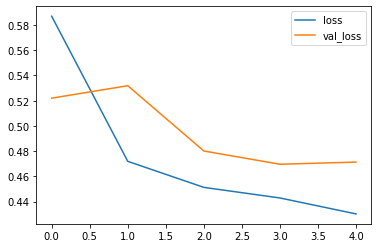
训练集的损失值一直下降,但是验证测试集的损失值,开始下降,后面反而升高
将正确率绘制成图像
plt.plot(history.epoch,history.history.get('acc'),label='acc')
plt.plot(history.epoch,history.history.get('val_acc'),label='val_acc')
plt.legend()
plt.show()
显示效果如下图: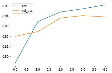
训练集的正确率下降,但是验证测试集的正确率,开始下降,后面反而升高